인과추론의 데이터과학. (2021, Nov 29). [Session 18-1] 가상의 통제집단 (Synthetic Control) [Video]. YouTube.
인과추론의 데이터과학. (2021, Nov 29). [Session 18-2] 가상의 통제집단 분석 사례 [Video]. YouTube.
인과추론의 데이터과학. (2021, Dec 6). [Session 18-3] 데이터 기반의 인과관계 발견 (Causal Discovery) [Video]. YouTube.
Session 18-1
- synthetic control: 여러 요인들을 결합해서 만든 합성의 control group
- counterfactual을 모방하기 위해 만든 것
- Causal effect
- ITE(individual treatment effect)는 구하기 어려움 → ATE활용
- 인과추론의 목표: ATET 추론
- Average Treatment Effect on the Treated
- Ignorability = Exchangeability = Unconfoundedness = Exogeneity
- treatment, control group이 treatment를 제외한 모든 것이 동일해야 함
- PO: Ceteris Paribus
- SCM: Backdoor/Frontdoor Criterion
Panel Data
- Panel Data: treatment 전후의 관측 데이터
- 시간에 대한 인과 관계를 조사하고 모델링하는 데 사용됨
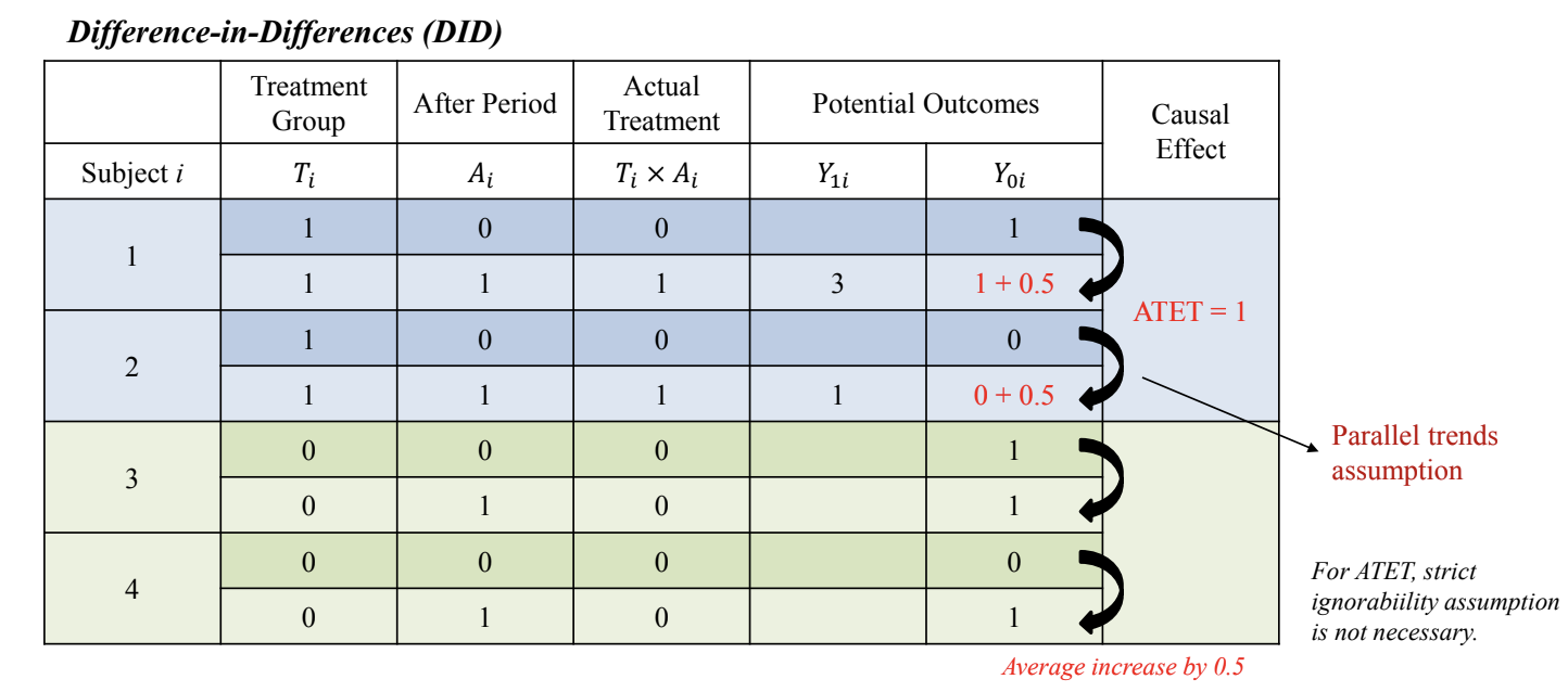
- DID(Difference-in-Differences) 활용
- ATET를 구하는 것이 목적
- treatment의 counterfactual을 구하는 것이 목표
- treatment 이전의 변수들을 활용
- 시간에 따라 변하지 않는 요인들을 반영할 수 있음 → treatment가 없었을 때, 즉 counterfactual을 구할 수 있음
- e.g. 아래 그림에서 파란색 (1, 0) 값을 그대로 가져오는 부분
- Parallel trends assumption:
- Ignorability보다 느슨한 가정
- 정의: treatment, control 그룹은 동일한 추세를 가지고 있어야 함
- treatment 이후에도 treatment 그룹과 control group은 변화 패턴이 유사하게 유지되어야 함
- e.g. 아래 그림에서 초록색 Subject 3,4의 평균 변화량 0.5를 그대로 가져오는 부분
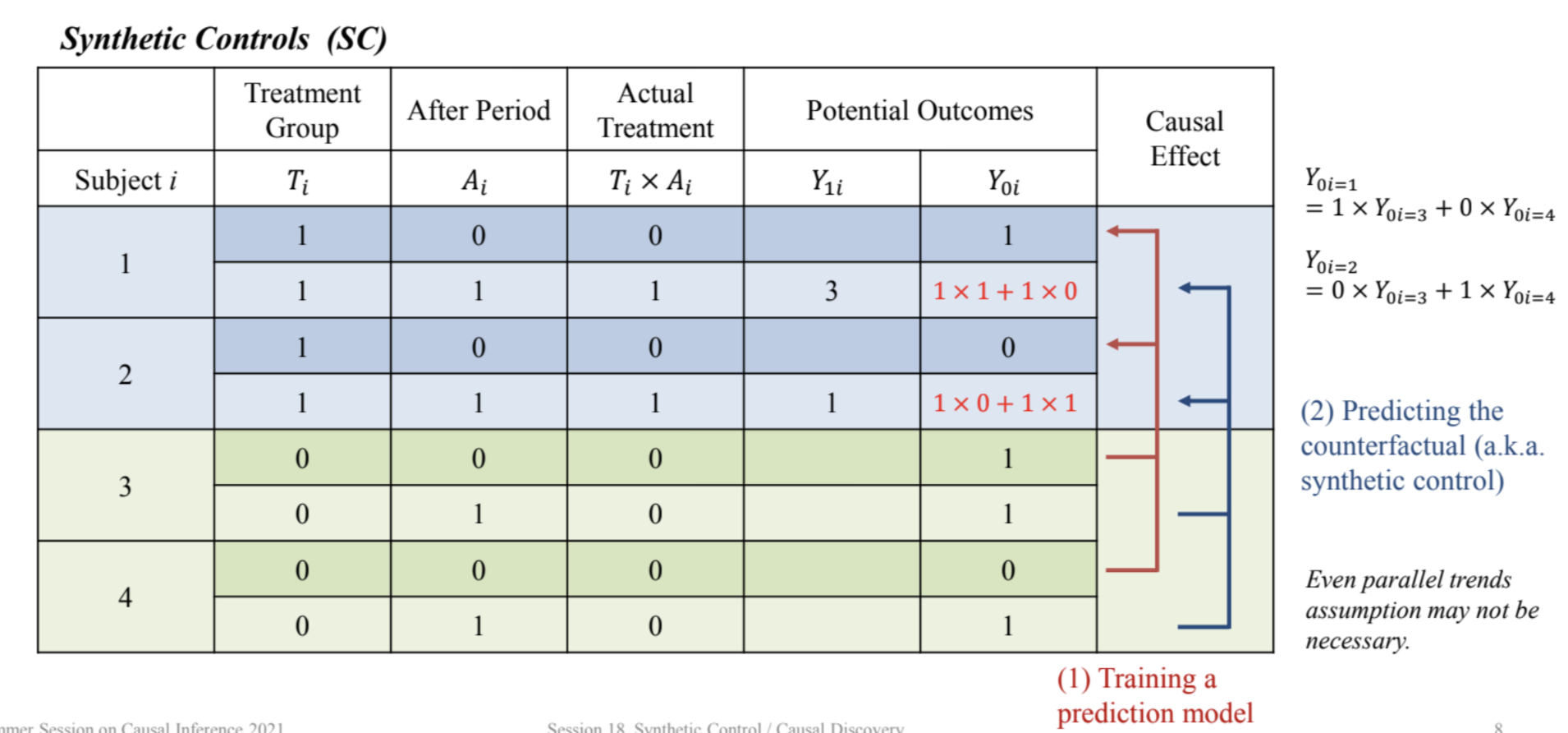
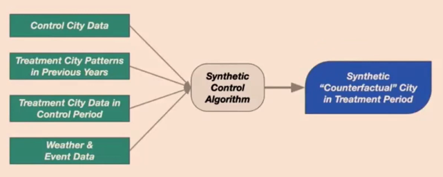
Synthetic Control (SC)
- control 그룹의 조합을 통해서 treatment의 counterfactual을 예측하는 것이 목적
- control group의 변수를 활용
- DID의 확장 + 유연한 방법
- 여러 가지 prediction을 할 수 있음
- 별도의 가정이 필요 없음
- ATET까지는 충분히 구할 수 있다는 idea
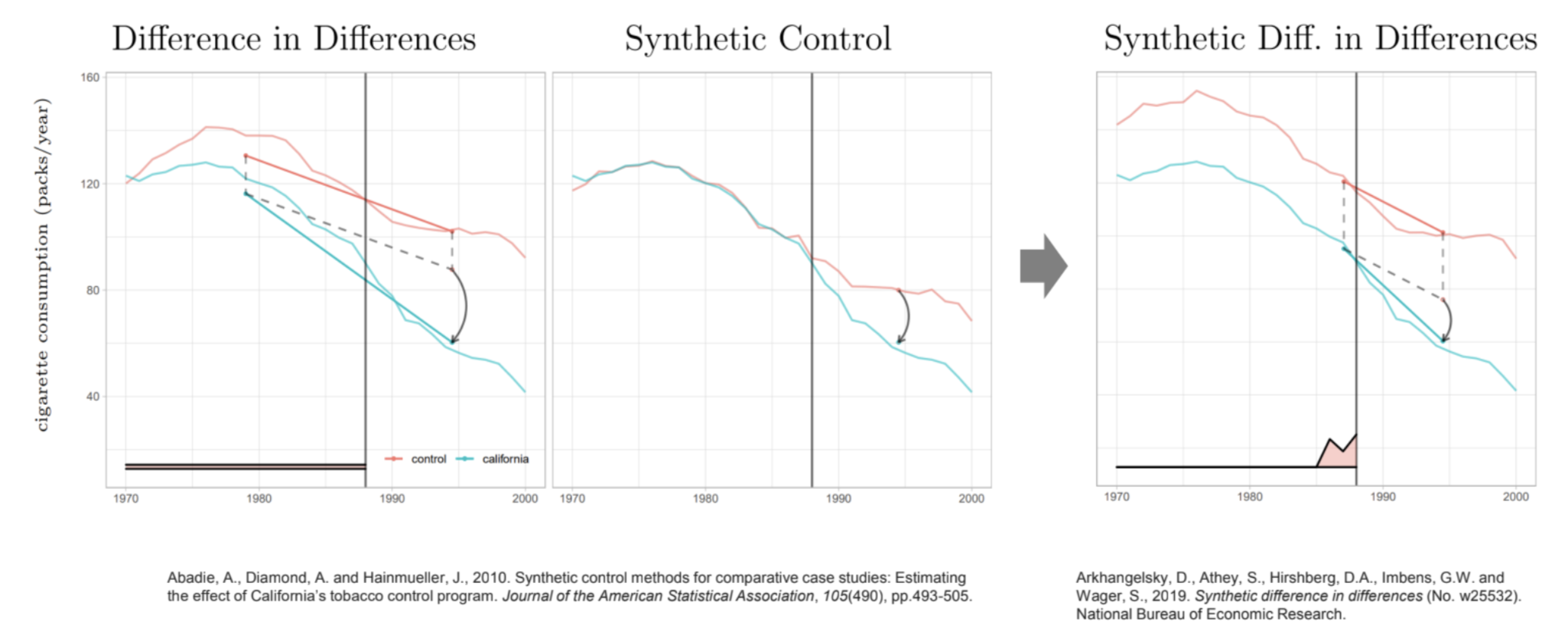
Case 1. Impact of California Anti-Tobacco Legislation
- treatet unit: California
- 1970s 후반부터 parallel 함
- fixed effect: 절댓값이 중요하지 않고 trend만 중요한 부분 → 시간에 따라 변하지 않는 효과
- 패널 데이터의 특성을 고려하고 인과관계를 더 정확하게 추론하는 데 도움을 줌
- 개체 간의 고유한 특성을 제어하여 개체 내 or 시간 내의 변동성을 고려한 회귀 분석을 수행할 수 있음
- DID에서 중요한 부분
- Synthetic DID: DID의 fixed effect + Synthetic control의 control unit의 weight을 고려한 방법
Session 18-2
Case 2. Impact of Reunification on West Germany
- reunification의 counterfactual를 유사한 국가를 통합하여 모방한 사례
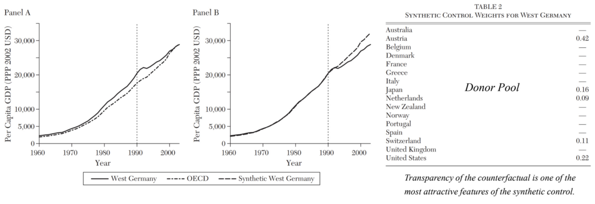
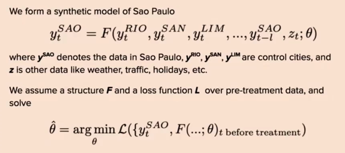
How to Construct the Synthetic Control
- original method: 결과를 직접적으로 예측하기보다 간접적인 방법을 채택
- predictor를 모방하는 모델을 만드는 것
- Case 2 기준, inflation rate, 산업 구조, 교육 수준을 모방하는 synthetic control를 만드는 것
- predictor의 weight과 control group의 weight을 최적화하는 문제
- Instead of predicting the outcome directly, it aims to choose weights of control units to minimize the difference in the pre-intervention values of predictors of the outcome
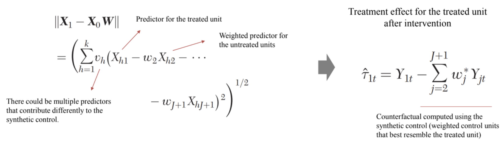
- 다양한 방법이 있음 (e.g. Lasso, Elastic net ..)
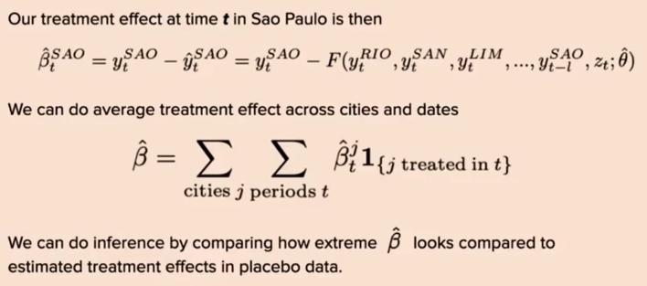
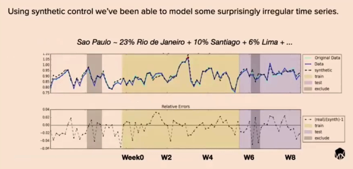
- 궁극적으로 synthetic control의 큰 목적은 out-of-sample prediction이다.
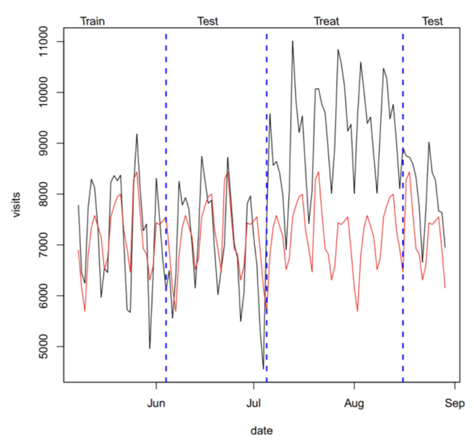
Sensitivity Tests for Synthetic Controls
- train-test split 접근 활용
- Train – Test – Treat – Compare (TTTC) process
What if There is No Control Group?
- DID, Synthetic control 적용 불가능
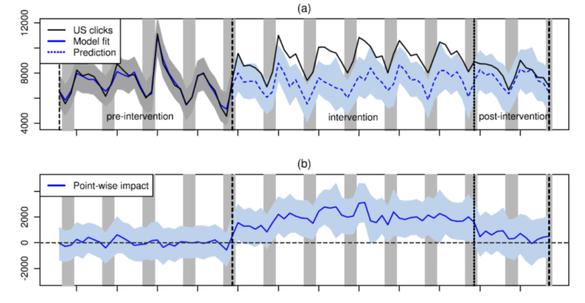
- time-series forecasting model을 활용하여 counterfactual을 예측
- data
- pre-intervention data → train
- intervention data → test
- post-intervention data → predict
- 구조적인 변화는 유추할 수 없기 때문에, time-series는 한계가 있음
- control group이 없는 상황에서는 time-series model을 최후의 보루로 사용하는 것을 권장
Case 3. Uber’s Application of Synthetic Control
- Problems
- Uber operate in cities with few credit cards
- difficulties in change and drivers paying service fees
- Why are A/B tests not feasible in some cases?
- experiment: tell drivers if a trip is cash
- hypothesis: some drivers don't like cash trips because of the change
- want to know
- trip acceptance rates
- unpaid service fees
- Spillover effects: treatment applied to one group affects the other group
- turns out drivers preferred cash trips -> declined more credit card trips
- control group received those trips that the treatment group declined
- experiment: tell drivers if a trip is cash
- Alternative to A/B test
- Difference-in-differences across cities
- Synthetic control across cities
- Main idea of Synthetic control
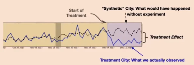
- Form
- Estimate treatment effect
- Result - actually works
Case 4. Causal Analysis of GS25 vs CU
Requirements
- Contextual Requirements
- Size of the Effect and Volatility of the Outcome
- Availability of a Comparison Group
- No Anticipation
- No Interference
- Convex Hull Condition
- Time Horizon
- Data Requirements
- Aggregate Data on Predictors and Outcomes
- Sufficient Pre-intervention Information
- Sufficient Post-intervention Information
- Reference: Using Synthetic Controls: Feasibility, Data Requirements, and Methodological Aspects
Session 18-3
Causal Discovery
- knowledge discovery
- theory → evidence (data)
- evidence (data) → theory
- ex. 케플러 데이터 패턴을 통해 인과관계를 도출
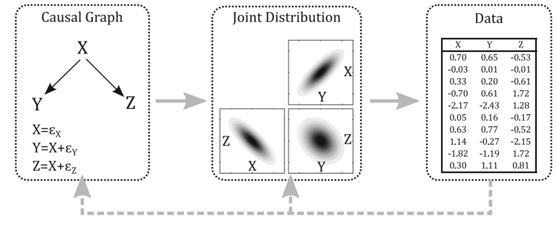
- Data generation process: causal graph → data
- causal discovery: data → causal graph
- Overall Structure
Causal Markov and Faithfulness Assumptions
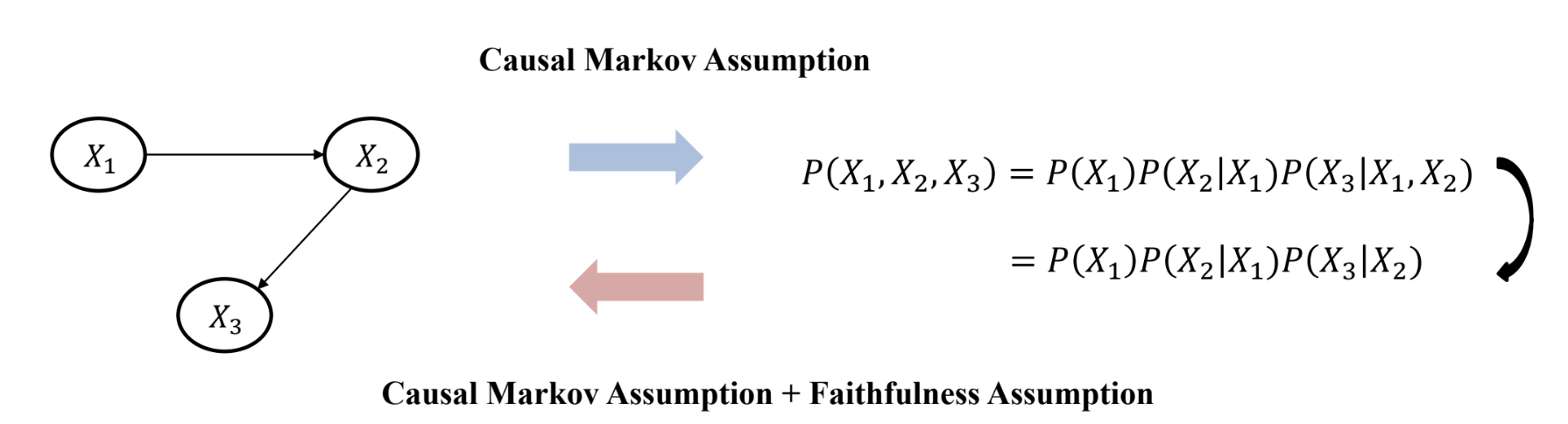
- Causal Markov Assumption: A node is dependent only on its descendants in the graph
- a node is independent on other variables, conditional on its causes
- Faithfulness Assumption: Nodes that are causally connected in a particular way in the graph are probabilistically dependent.
- 인과적으로 연결되어 있으면 확률적으로 dependent해야 함
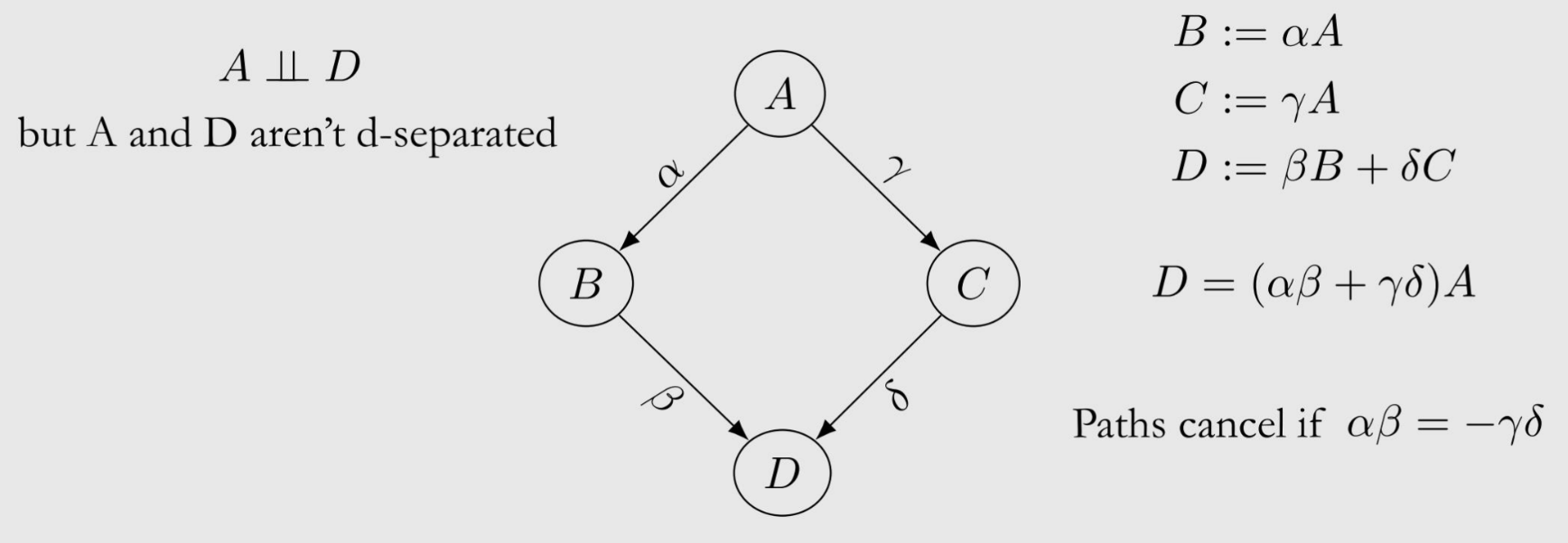
- Violation of Faithfulness Assumption
- Distinct causal paths that have opposite effects could cancel out each other.
- e.g. A→B→D (+1), A→C→D (-1)이면, 효과가 상쇄됨
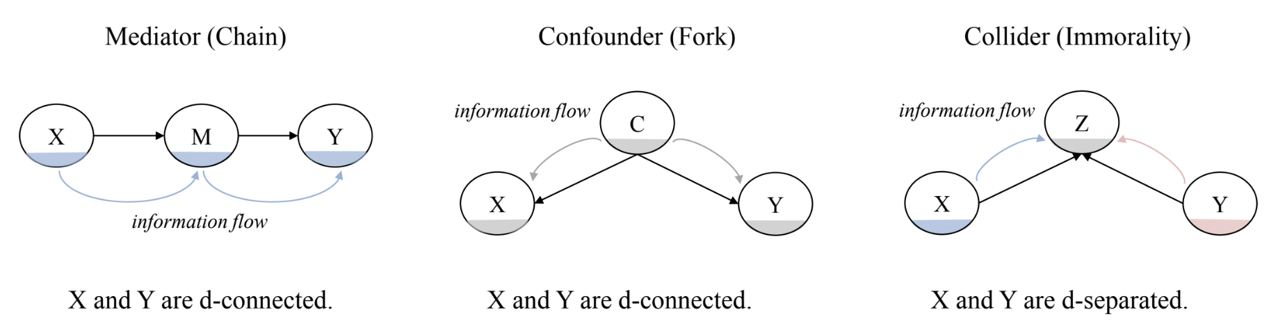
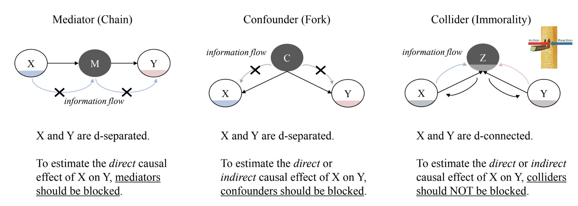
Conditional (In-)Dependence (Association)
- Association이 없다 = de-seperated = independence
- Before conditioning
- chain, fork → dependent
- immorality → independent
- After conditioning
- chain, fork → independent
- immorality → dependent
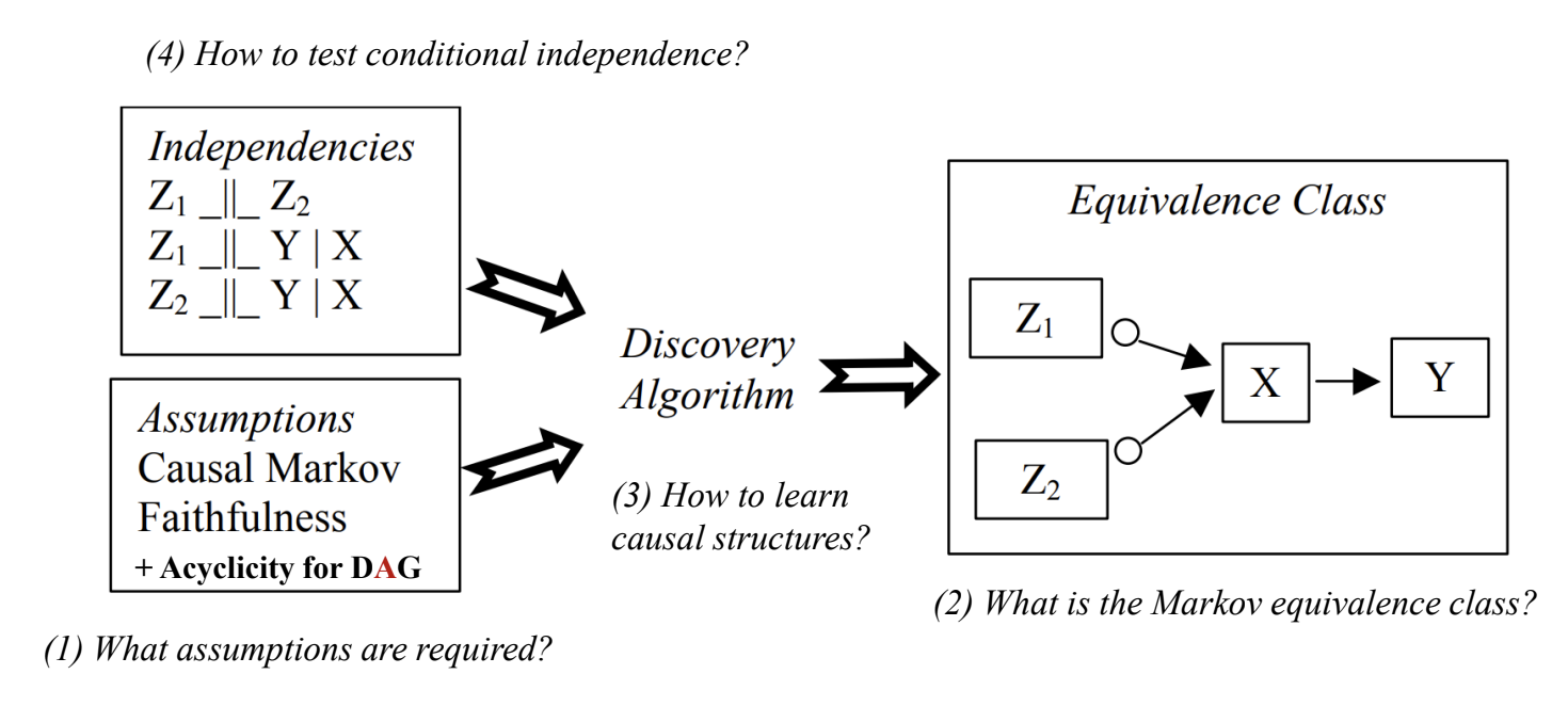
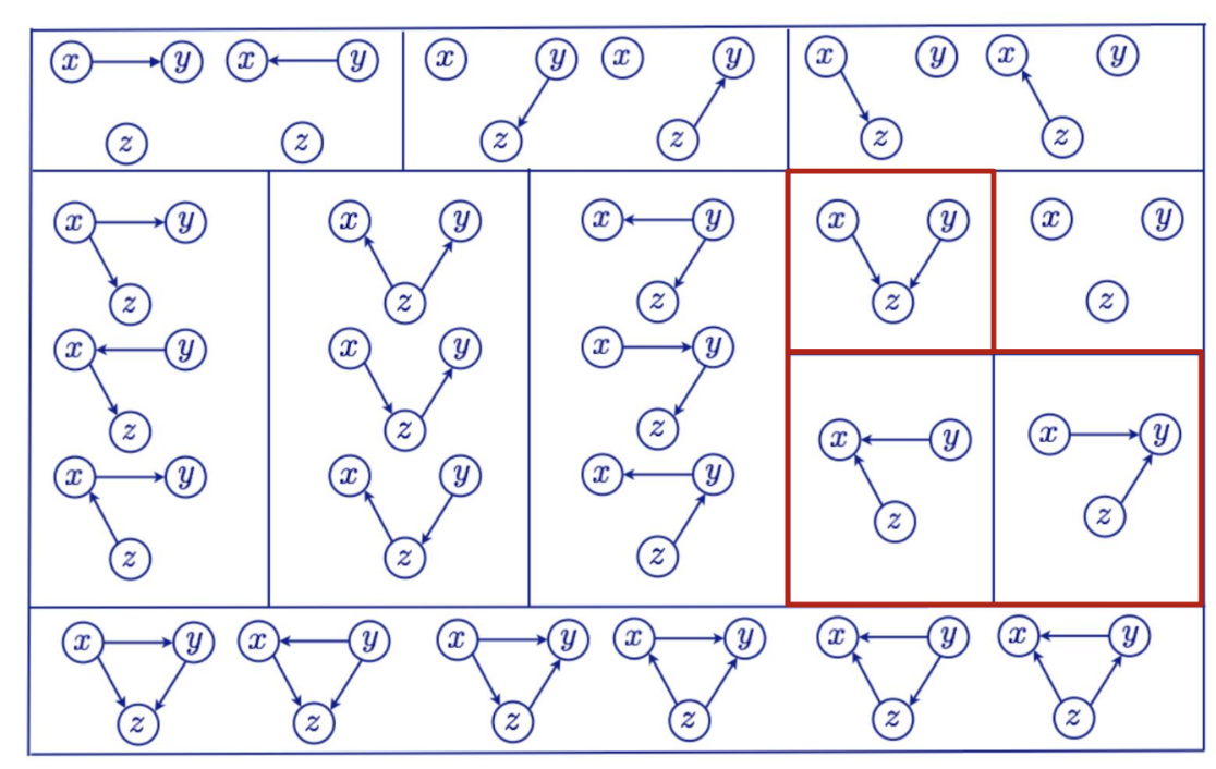
Markov Equivalence Class
- A set of DAGs that encode the same set of conditional independencies.
- 동일한 conditional independencies를 갖는 graph들의 class를 의미
- “V” structures (= colliders = immorality) → 핵심적인 역할을 함
- has only one structure for the same class
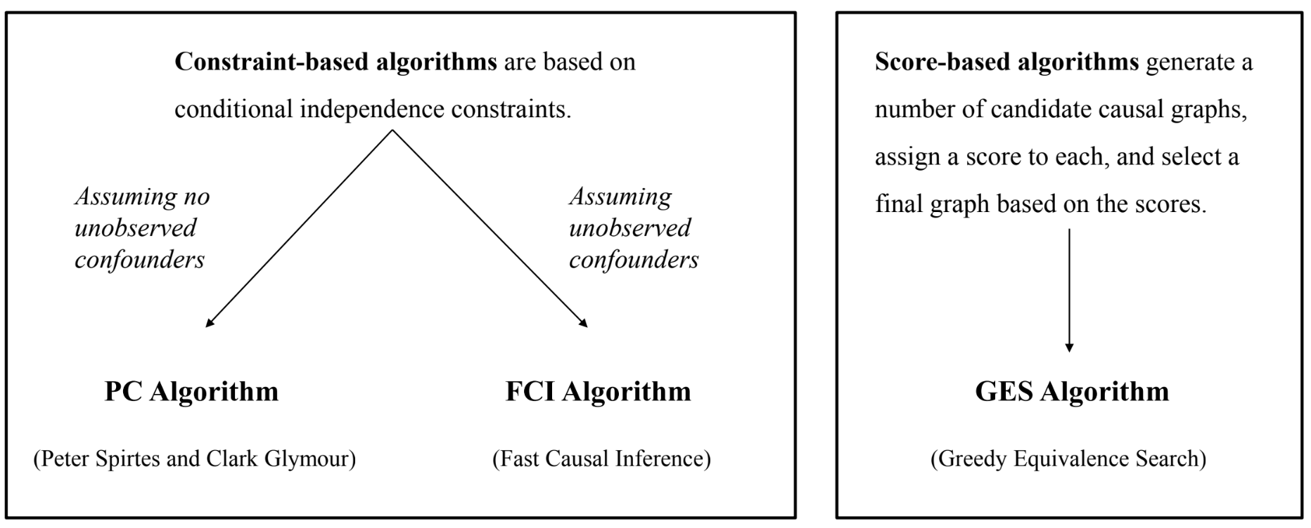
Causal Discovery Algorithms
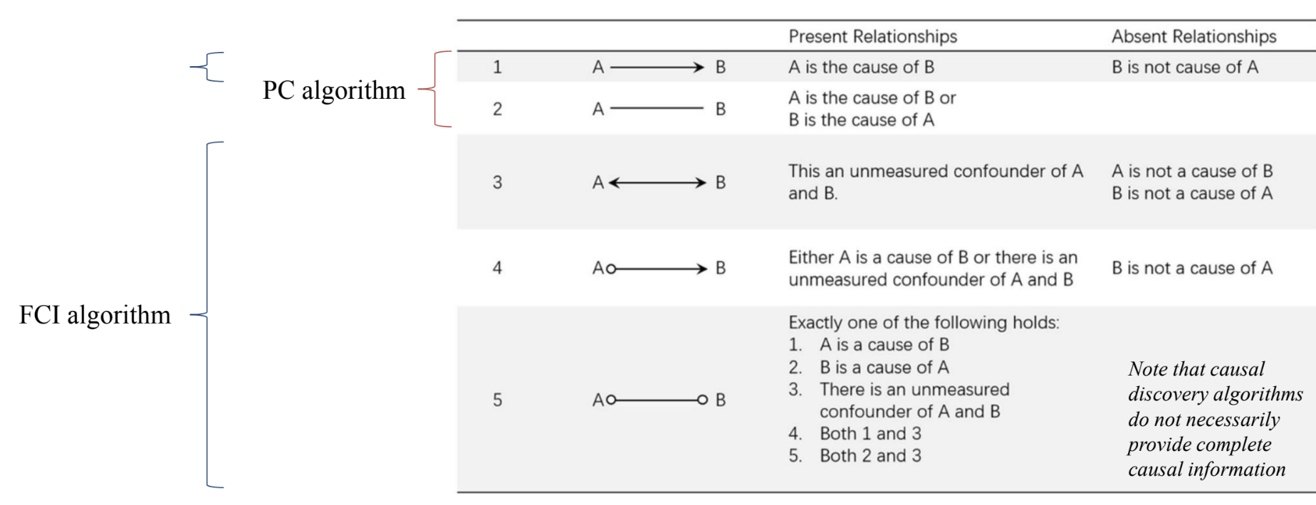
- Constraint-based algorithms
- PC algorithm: assume no unobserved confounders
- FCI algorithm: assume unobserved confounders
- Score-based algorithms → score를 maximize
- GES algorithm
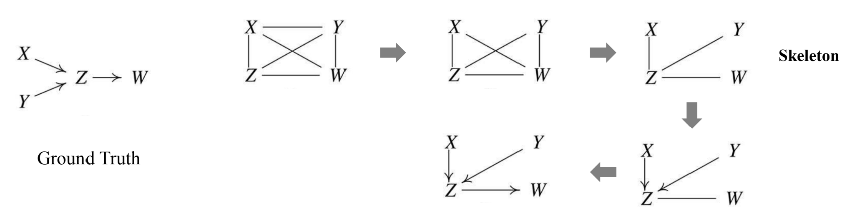
1. PC Algorithm
- Step 1. Start with a complete undirected graph.
- Step 2. Eliminate edges between variables that are unconditionally independent.
- X. Y는 independent함 → eliminate
- Step 3. For each pair of variables having an edge between them, eliminate the edge if they are independent, conditional on a subset of variables with edges to them (increasing the size of subsets 1 to n).
- X, W 사이에는 direct path가 없음 → eliminate
- Y, W 사이에는 direct path가 없음 → eliminate
- Step 4. Identify a “V” structure (collider, immorality) and orient edges.
- Step 5. Orient the remaining edges not to be a collider (i.e., orientation propagation).
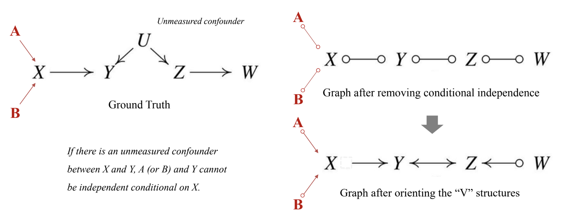
2. FCI Algorithm
- similar to PC algorithm
- further assumes that there could be an unmeasured confounder between nodes
- except the “Y” structures
- y structure가 있는 부분에서는 unmeasured confounter가 없음
- 양방향 화살표가 가능함
- except the “Y” structures
3. GES Algorithm
- 빈 graph에서 시작해서 greedy하게 진행하는 방식
- Step 1. Start with an empty graph containing no edges.
- Step 2. Greedily add edges (dependencies) one at a time in the orientation that maximize some fit score, such as Bayesian Information Score (BIC) (the lower, the better fit).
- Step 3. Map the resulting model to the corresponding Markov equivalence class.
- Step 4. Continue Steps 2 and 3 until the score can no longer be improved.
- Step 5. Remove edges one at a time as long as it maximizes the score (e.g., decreases the BIC).
- Step 6. Continue Step 5 until no further edges can be removed.
Conditional Independence Tests
- Bayesian networks (causal graph)에서 variable의 distribution이 중요함
- type
- Discrete Bayesian networks (categorical variables)
- Discrete Bayesian networks (ordered factors)
- Gaussian Bayesian networks (continuous normal variables)
- Non-Gaussian Bayesian networks (continuous variables)
Practical Guidance for Causal Discovery
- Causal discovery algorithms work asymptotically (i.e., with a large volume of data)
- Distributions of the variables play a critical role in conditional independence tests
- Domain knowledge may help the causal discovery
반응형
'Causal inference' 카테고리의 다른 글
| Chapter 1. 인과-행동 프레임워크 (0) | 2023.11.24 |
|---|---|
| [KSSCI 2021] 인과추론의 데이터 과학 - Session 5 (0) | 2023.10.16 |
| Part 5. Advanced Topics for Analyzing Experiments (0) | 2023.10.12 |
| [KSSCI 2021] 인과추론의 데이터 과학 - Session 17 (0) | 2023.10.12 |
| [KSSCI 2021] 인과추론의 데이터 과학 - Session 12 (1) | 2023.10.11 |


댓글