Chapter 8. 비지도 학습: 토픽 모델링 및 클러스터링

젠스 알브레히트, 시다르트 라마찬드란, 크리스티안 윙클러, 『파이썬 라이브러리를 활용한 텍스트 분석 Blueprints for Text Analytics Using Python』, 심상진, 한빛미디어-OREILLY(2022), p281-320.

NMF (Non-negative Matrix Factorization)

비음수 행렬 분해
선형대수 기반 방법론
문서-용어 행렬의 인수분해로 문서 말뭉치에서 잠재 구조를 가장 쉽게 찾을 수 있음
- 문서-용어 행렬은 양수 값 요소만 있어서 NMF 활용 가능
\(V\approx W\cdot H\)
- V: 문서 * 단어
- W: 문서 * 토픽
- H: 토픽 * 단어
구현
- sklearn.decomposition.NMF 활용
- 임의의 주제 개수를 선택 (n_components)
- 각 토픽별 단어의 백분율이 급격히 낮아지면 주제가 잘 정의됐다고 볼 수 있음
- 문서에 대한 주제 기여도의 총합을 정규화하여 균일하게 분포하는지 비교
  - 만약 특정 주제가 큰 기여를 하는 경우 주제 개수를 조정해야 함

from sklearn.decomposition import NMF

nmf_text_model = NMF(n_components=10, random_state=42)
W_text_matrix = nmf_text_model.fit_transform(tfidf_text_vectors)
H_text_matrix = nmf_text_model.components_

def display_topics(model, features, no_top_words=5):
    for topic, words in enumerate(model.components_):
        total = words.sum()
        largest = words.argsort()[::-1] # invert sort order
        print("\nTopic %02d" % topic)
        for i in range(0, no_top_words):
            print("  %s (%2.2f)" % (features[largest[i]], abs(words[largest[i]]*100.0/total)))

display_topics(nmf_text_model, tfidf_text_vectorizer.get_feature_names_out()) # 주제별 중요한 단어 확인
W_text_matrix.sum(axis=0)/W_text_matrix.sum()*100.0 # 문서의 주제 기여도 총합 정규화

SVD (Singular-Value Decomposition)

특잇값 분해
선형대수 기반 방법론
문서-용어 행렬에서 블록 구조를 찾아내는 방식으로 문서와 단어를 재배치한 것
- Full SVD 케이스는 사용하는 경우가 드물기 때문에 차원을 줄인 형태인 Truncated SVD를 활용

\(V=U\cdot \sum\cdot V^*\)
- \(U\): m x m (문서 * 토픽)
- \(\sum\): m x n (특잇값; 대각행렬)
- \(V^*\): n x n (특잇값 * 단어)

from sklearn.decomposition import TruncatedSVD

svd_para_model = TruncatedSVD(n_components = 10, random_state=42)
W_svd_para_matrix = svd_para_model.fit_transform(tfidf_para_vectors)
H_svd_para_matrix = svd_para_model.components_

display_topics(svd_para_model, tfidf_para_vectorizer.get_feature_names_out())
svd_para_model.singular_values_ # 주제별 기여도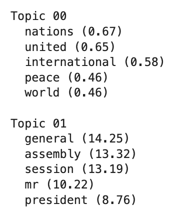

LDA (Latent Dirichlet Allocation)

잠재 디리클레 할당
확률론적 방법론
각 문서에 서로 다른 주제가 혼합되어 있다고 생각하는 방법
이론
- 문서당 주제의 수를 적게 유지하고 주제를 구성하는 중요한 단어 몇 개만 포함하기 위해 디리클레 분포를 사용
  - Dirichlet distribution = Dirichlet prior
  - 디리클레 분포는 문서에 주제를 할당할 때, 주제에 대한 단어를 찾을 때 모두 적용됨
- 주제와 단어에 대해 디리클레 분포를 따른다고 가정
- 분포를 따르도록 확률적 샘플링(stochastic sampling)을 통해 원본 문서에서 단어를 다시 생성
- 절차가 여러 번 반복되어야해서 계산 집약적임
구현
- sklearn.decomposition.LatentDirichletAllocation 활용

from sklearn.decomposition import LatentDirichletAllocation

lda_para_model = LatentDirichletAllocation(n_components = 10, random_state=42)
W_lda_para_matrix = lda_para_model.fit_transform(count_para_vectors)
H_lda_para_matrix = lda_para_model.components_

display_topics(lda_para_model, count_para_vectorizer.get_feature_names_out())
W_lda_para_matrix.sum(axis=0)/W_lda_para_matrix.sum()*100.0 # 주제별 기여도

LDA 시각화
- pyLDAvis.lda_model 활용
- 주제의 차원 축소 방법: mds 매개변수 활용
  - “pcoa”(PCA), “tsne”(T-SNE), “mmds”(Metric Multidimensional Scaling) 선택 가능
  - T-SNE 활용 시, 주제 간 거리 맵이 변경되고 겹치는 주제의 버블이 PCA보다 더 적게 표시됨
  - 2차원 벡터로 투영된 결과일 뿐, 주제 단어 분포의 경향성 정도만 파악하는 것을 권장

import pyLDAvis.lda_model

lda_display = pyLDAvis.lda_model.prepare(lda_para_model, count_para_vectors, count_para_vectorizer, sort_topics=False)
pyLDAvis.display(lda_display)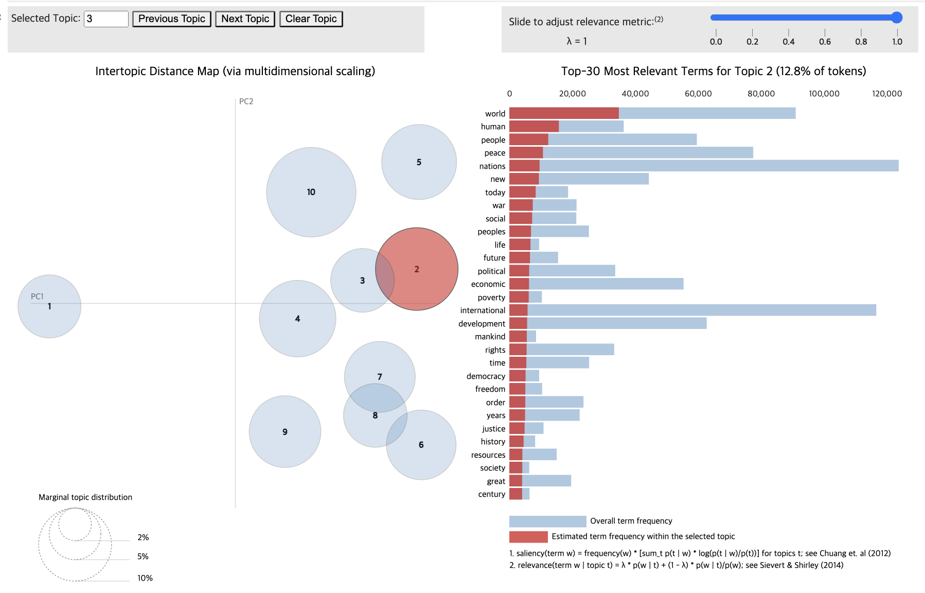

Wordcloud

토픽 모델 시각화 방법
워드 클라우드는 각 주제별 개별 스케일링을 사용함

%matplotlib inline
import matplotlib.pyplot as plt
from wordcloud import WordCloud

def wordcloud_topics(model, features, no_top_words=40):
    for topic, words in enumerate(model.components_):
        size = {}
        largest = words.argsort()[::-1] # invert sort order
        for i in range(0, no_top_words):
            size[features[largest[i]]] = abs(words[largest[i]])
        wc = WordCloud(background_color="white", max_words=100, width=960, height=540)
        wc.generate_from_frequencies(size)
        plt.figure(figsize=(12,12))
        plt.imshow(wc, interpolation='bilinear')
        plt.axis("off")
        # if you don't want to save the topic model, comment the next line
        plt.savefig(f'topic{topic}.png')

wordcloud_topics(nmf_para_model, tfidf_para_vectorizer.get_feature_names_out())

시간에 따른 토픽 분포 변화 추이

토픽 분포가 시간의 경과에 따라 어떻게 변하는지 확인하는 것이 좋다

from tqdm.auto import tqdm
import numpy as np
import matplotlib.pyplot as plt

year_data = []
for year in tqdm(np.unique(np.unique(paragraph_df["year"]))):
    W_year = nmf_para_model.transform(tfidf_para_vectors[np.array(paragraph_df["year"] == year)])
    year_data.append([year] + list(W_year.sum(axis=0)/W_year.sum()*100.0))

topic_names = []
voc = tfidf_para_vectorizer.get_feature_names()
for topic in nmf_para_model.components_:
    important = topic.argsort()
    top_word = voc[important[-1]] + " " + voc[important[-2]]
    topic_names.append("Topic " + top_word)

df_year = pd.DataFrame(year_data, columns=["year"] + topic_names).set_index("year")
df_year.plot()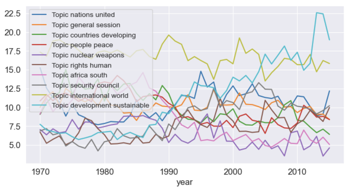

Gensim

파이썬의 대표적인 토픽 모델링 수행 도구
구현
- 토큰화된 데이터 (문서)를 준비해야 함
  - 젠심에는 통합된 토큰화가 없음
- 토큰화된 문서들로 젠심 사전을 초기화
- 단어 가방 행렬 (젠심에서 말뭉치로 불림) 계산
- TF-IDF 변환 수행
- NMF, LDA 실행 및 분포 확인
  - NMF는 coherence score (일관성 점수)로 품질을 확인
  - LDA는 perplexity로 품질을 확인
    - perplexity: 확률 모델이 샘플을 얼마나 잘 예측하는지 측정
- NMF(coherence score), LDA(perplexity) 별 최적의 주제 수를 찾기
  - 각 방법별 점수를 최대화하는 토픽 수 추출
  - LDA 모델은 계산 비용이 많이 들기 대문에 최소한의 모델과 복잡성만 계산하도록 설정 필요
  - 너무 많은 주제를 선택할 경우, 해석이 어려워짐
  - 일관성 점수가 높다고 해석이 명확한 것은 아님을 주의하자

from gensim.corpora import Dictionary
from gensim.models import TfidfModel
from gensim.models.nmf import Nmf
from gensim.models import LdaModel
from gensim.models.coherencemodel import CoherenceModel

dict_gensim_para = Dictionary(gensim_paragraphs) # 토큰화된 문서들로 젠심 사전을 초기화
dict_gensim_para.filter_extremes(no_below=5, no_above=0.7) # 어휘 줄이기 (최소 5개 문서 등장, 총 문서의 70% 초과하지 않도록 설정한 예시)
bow_gensim_para = [dict_gensim_para.doc2bow(paragraph) for paragraph in gensim_paragraphs]

# TF-IDF 변환
tfidf_gensim_para = TfidfModel(bow_gensim_para) 
vectors_gensim_para = tfidf_gensim_para[bow_gensim_para]

# 토픽별 젠심 모델의 분포 확인
def display_topics_gensim(model):
    for topic in range(0, model.num_topics):
        print("\nTopic %02d" % topic)
        for (word, prob) in model.show_topic(topic, topn=5):
            print("  %s (%2.2f)" % (word, prob))

# NMF 실행
nmf_gensim_para = Nmf(vectors_gensim_para, num_topics=10, id2word=dict_gensim_para, kappa=0.1, eval_every=5, random_state=42)
display_topics_gensim(nmf_gensim_para) # 위에서 첨부했던 예시 이미지와 유사한 방식
## coherence score 계산
nmf_gensim_para_coherence = CoherenceModel(model=nmf_gensim_para, texts=gensim_paragraphs, dictionary=dict_gensim_para, coherence='c_v')
nmf_gensim_para_coherence_score = nmf_gensim_para_coherence.get_coherence()
print(nmf_gensim_para_coherence_score) 

# LDA 실행
lda_gensim_para = LdaModel(corpus=bow_gensim_para, id2word=dict_gensim_para, chunksize=2000,
    alpha='auto', eta='auto', iterations=400, num_topics=10, passes=20, eval_every=None, random_state=42)
display_topics_gensim(lda_gensim_para) # 위에서 첨부했던 예시 이미지와 유사한 방식
## perplexity 계산
lda_gensim_para_coherence = CoherenceModel(model=lda_gensim_para, texts=gensim_paragraphs, dictionary=dict_gensim_para, coherence='c_v')
lda_gensim_para_coherence_score = lda_gensim_para_coherence.get_coherence()
print(lda_gensim_para_coherence_score)

# LDA 최적의 주제 수 찾기
from gensim.models.ldamulticore import LdaMulticore

lda_para_model_n = []
for n in tqdm(range(5, 21)):
    lda_model = LdaMulticore(corpus=bow_gensim_para, id2word=dict_gensim_para, chunksize=2000,
                             eta='auto', iterations=400, num_topics=n, passes=20, 
                             eval_every=None, random_state=42)
    lda_coherence = CoherenceModel(model=lda_model, texts=gensim_paragraphs, 
                                   dictionary=dict_gensim_para, coherence='c_v')
    lda_para_model_n.append((n, lda_model, lda_coherence.get_coherence()))

pd.DataFrame(lda_para_model_n, columns=["n", "model", "coherence"]).set_index("n")[["coherence"]].plot(figsize=(16,9))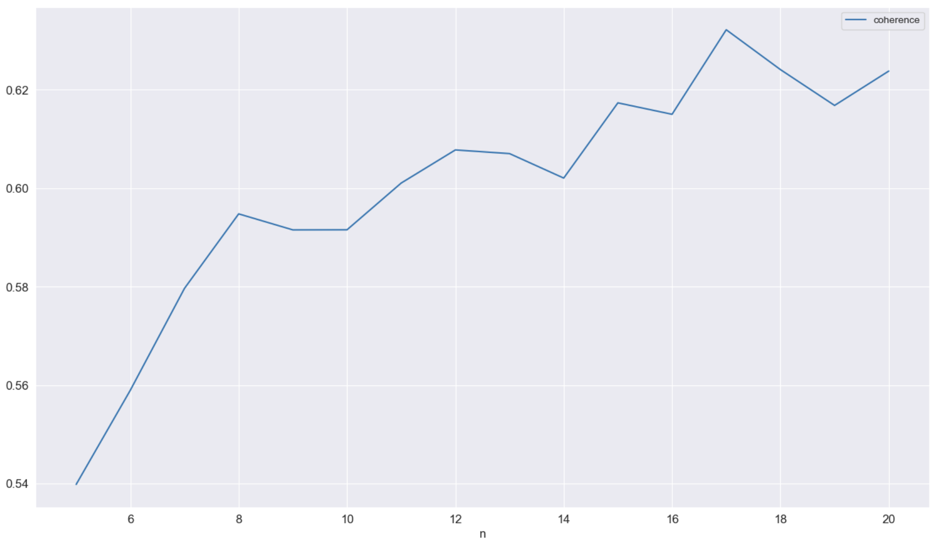

HDP (Hierarchical Dirichlet Process)

계층적 디리클레 절차
넓은 주제를 제공하고, 하위 주제를 제공하는 방식
- 잘 구분된 몇 가지 광범위한 주제를 제공한 후 더 많은 단어를 추가하고, 주제 정의를 더 차별화함

from gensim.models import HdpModel
import re

hdp_gensim_para = HdpModel(corpus=bow_gensim_para, id2word=dict_gensim_para)

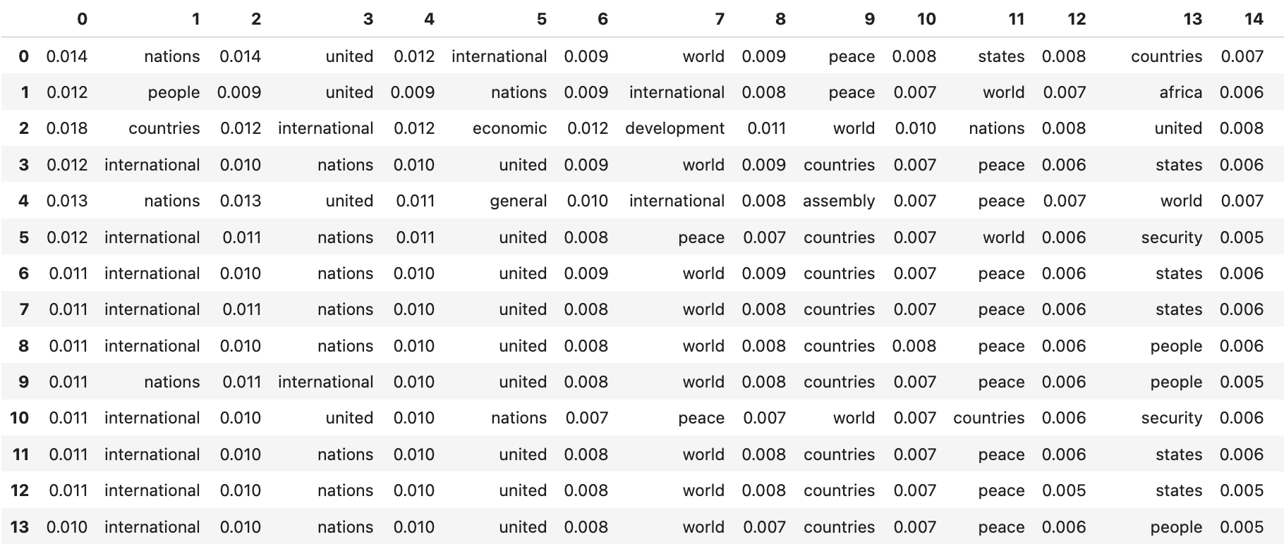
words = 8
pd.DataFrame([re.split(r" \+ |\*", t[1]) for t in hdp_gensim_para.print_topics(num_topics=20, num_words=words)])

hdp_gensim_para.show_topic(0, topn=10) # 주제별 Top10 단어 결과
"""
[('nations', 0.014275215007241408),
 ('united', 0.014068210031074795),
 ('international', 0.011670088475680272),
 ('world', 0.009430601473576466),
 ('peace', 0.008573897369285592),
 ('states', 0.00818353773344016),
 ('countries', 0.007844526055737289),
 ('security', 0.006645959516037016),
 ('general', 0.005334125248632264),
 ('nuclear', 0.0050745524616676915)]
"""

Clustering 방법

알고리즘: K-means, BIRCH, spectral clustering
- BIRCH: Balanced Iterative Reducing and Clustering using Hierarchies
LDA보다 더 많은 시간이 걸리는 단점이 있음
데이터가 이질적인 경우, 대부분의 클러스터는 작게 생성되고 (작은 어휘 포함) 나머지를 모두 흡수하는 큰 클러스터가 존재함 → 클러스터 간 분포 확인 필요
품질 측정 방법: coherence score, Calinski-Harabasz score (칼린스키-하라바츠 점수) 활용

Reference

저작자표시 비영리 변경금지

'NLP' 카테고리의 다른 글

Chapter 7. 텍스트 분류기 (0)	2023.09.29
Chapter 6. 텍스트 분류 알고리즘 (0)	2023.03.26
Chapter 5. 특성 엔지니어링 및 구문 유사성 (0)	2023.03.26
Chapter 4. 통계 및 머신러닝을 위한 텍스트 데이터 준비 (0)	2023.03.26
Chapter 3. 웹사이트 스크래핑 및 데이터 추출 (0)	2023.03.26

NightFury

Chapter 8. 비지도 학습: 토픽 모델링 및 클러스터링

NMF (Non-negative Matrix Factorization)

SVD (Singular-Value Decomposition)

LDA (Latent Dirichlet Allocation)

Wordcloud

시간에 따른 토픽 분포 변화 추이

Gensim

HDP (Hierarchical Dirichlet Process)

Clustering 방법

Reference

'NLP' 카테고리의 다른 글

댓글

티스토리툴바

Chapter 8. 비지도 학습: 토픽 모델링 및 클러스터링

NMF (Non-negative Matrix Factorization)

SVD (Singular-Value Decomposition)

LDA (Latent Dirichlet Allocation)

Wordcloud

시간에 따른 토픽 분포 변화 추이

Gensim

HDP (Hierarchical Dirichlet Process)

Clustering 방법

Reference

'NLP' 카테고리의 다른 글

관련글

댓글

티스토리툴바